Day 7 Raster

Libraries

require(devtools)
devtools::install_github("ropensci/rerddap")
devtools::install_github("rmendels/rerddapXtracto") 

library(tidyverse)

── Attaching packages ─────────────────────────────────────── tidyverse 1.3.2 ──
✔ ggplot2 3.4.0      ✔ purrr   0.3.5 
✔ tibble  3.1.8      ✔ dplyr   1.0.10
✔ tidyr   1.2.1      ✔ stringr 1.4.1 
✔ readr   2.1.3      ✔ forcats 0.5.2 
── Conflicts ────────────────────────────────────────── tidyverse_conflicts() ──
✖ dplyr::filter() masks stats::filter()
✖ dplyr::lag()    masks stats::lag()

library(tidyterra)

Attaching package: 'tidyterra'

The following object is masked from 'package:stats':

    filter

Download sea surface temperature data

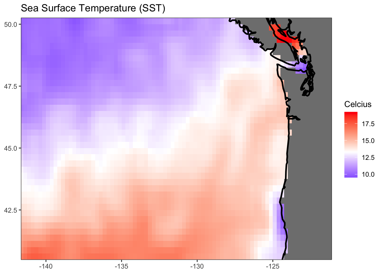
I will download the optimal interpolation sea surface temperature from CoastWatch. The bounding box is off the coast of Washington, USA.

filePath <- here::here("content", "data", "day7_sst_raster.RData")
lats <- c(40.375, 50.375)
lons <- c(-141.875, -120.875)
if (!file.exists(filePath)) {
df_info <- rerddap::info("ncdcOisst21Agg_LonPM180")
df <- rerddap::griddap("ncdcOisst21Agg_LonPM180", latitude = lats, longitude = lons, time = c("2021-06-19", "2021-06-19"), fields = "sst")$data
save(df, file=filePath)
}else{
  load(filePath)
}

Turn this into a raster. Need to tell raster that this is lat/long data.

df2 <- data.frame(x=df$lon, y=df$lat, z=df$sst)
ras <- raster::rasterFromXYZ(df2, crs = "+proj=longlat")

library(terra)

terra 1.6.17

Attaching package: 'terra'

The following object is masked from 'package:tidyr':

    extract

r <- terra::rast(ras)
names(r) <- "alt"
setMinMax(r)
slope <- terra::terrain(r, "slope", unit = "radians")
aspect <- terra::terrain(r, "aspect", unit = "radians")
hill <- terra::shade(slope, aspect, 10, 200)
names(hill) <- "shades"

library(scales)

Attaching package: 'scales'

The following object is masked from 'package:terra':

    rescale

The following object is masked from 'package:purrr':

    discard

The following object is masked from 'package:readr':

    col_factor

# Hillshading, but we need a palette
pal_greys <- hcl.colors(1000, "Grays")

index <- hill %>%
  mutate(index_col = rescale(shades, to = c(1, length(pal_greys)))) %>%
  mutate(index_col = round(index_col)) %>%
  pull(index_col)
# Get cols
vector_cols <- pal_greys[index]

hill_plot <- ggplot() +
  geom_spatraster(
    data = hill, fill = vector_cols, maxcell = Inf,
    alpha = 1
  )
hill_plot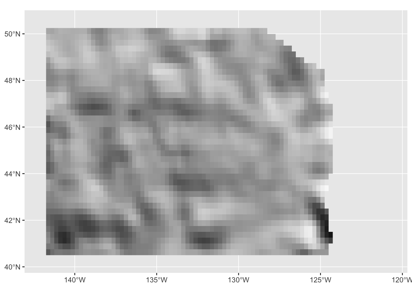

r_limits <- minmax(r) %>% as.vector()
# Rounded to lower and upper 500
#r_limits <- c(floor(r_limits[1] / 500), ceiling(r_limits[2] / 500)) * 500

base_plot <- hill_plot +
  geom_spatraster(data = r, maxcell = Inf) +
  scale_fill_hypso_tint_c(
    limits = r_limits,
    palette = "dem_poster",
    alpha = 0.4,
    labels = label_comma(),
    # For the legend I use custom breaks
    breaks = seq(-300, 1000, 100)
  )
base_plot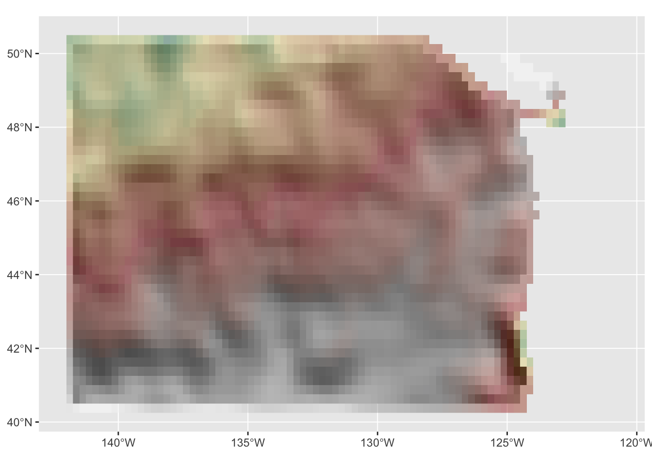

library(tidyterra)
hill_plot +
  geom_spatraster(data=r, maxcell = Inf) +
  scale_fill_hypso_tint_c(limits = as.vector(minmax(r)), 
                          palette = "etopo1",
                          alpha =0.4,
                          direction = 1,
                          labels = scales::label_comma()) +
  guides(fill=guide_legend(title = "elevation", reverse = FALSE))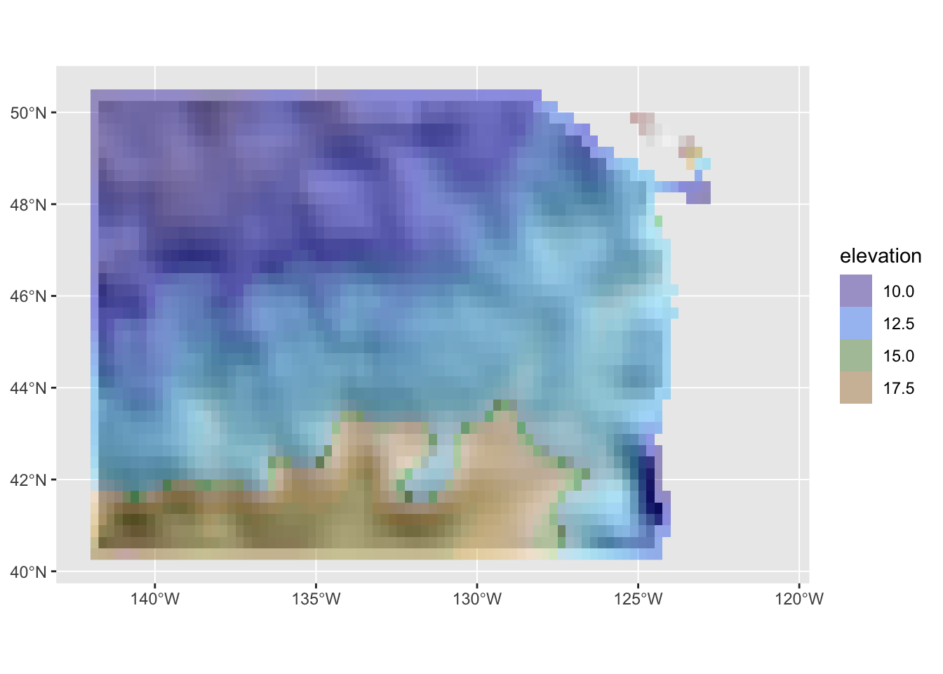

ggplot() + 
  geom_spatraster(data=slope, maxcell = Inf) +
  scale_fill_whitebox_c(palette = "muted", alpha = 0.9, direction = 1)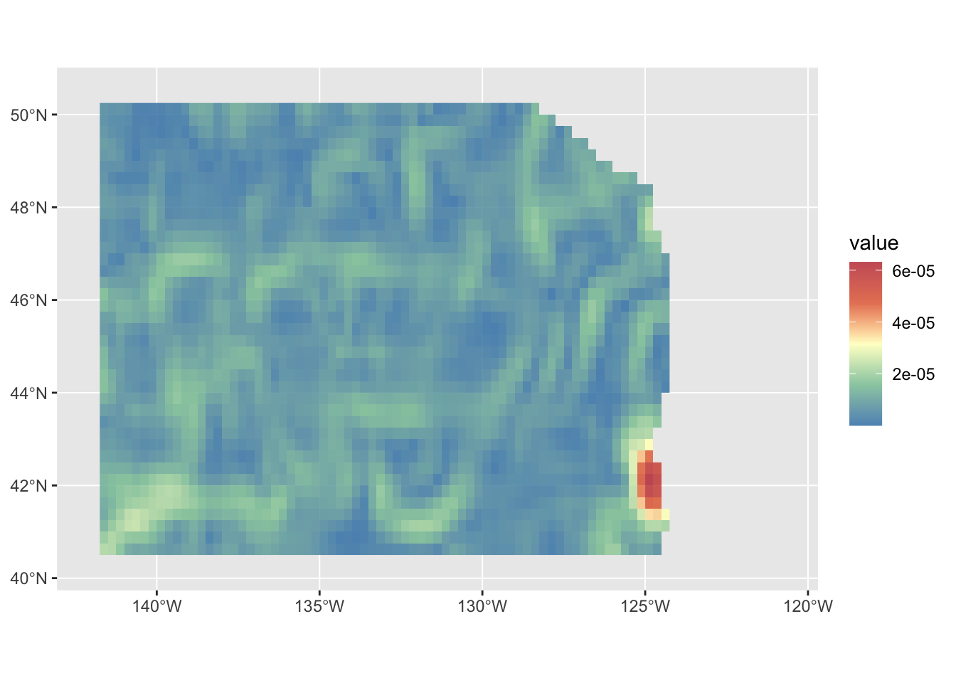

  geom_spatraster(data=r, maxcell = Inf) +
  scale_fill_whitebox_c(palette = "muted", alpha = 0.9, direction = 1)

NULL

library(colorspace)

Attaching package: 'colorspace'

The following object is masked from 'package:terra':

    RGB

hill_plot +
  geom_spatraster(data=r, maxcell = Inf) +
  scale_fill_continuous_diverging(
    palette = "Blue-Red-2", p2 = .1, alpha=.8, mid=mean(df$sst, na.rm = TRUE))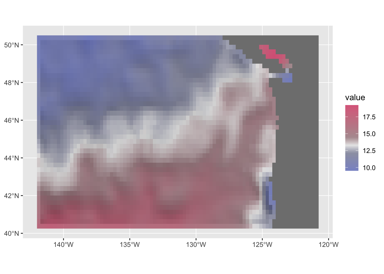

Plot the raster

library(raster)

Loading required package: sp

Attaching package: 'raster'

The following object is masked from 'package:tidyterra':

    select

The following object is masked from 'package:dplyr':

    select

library(ggplot2)
gg <- ggplot(df) +
  geom_raster(aes(longitude, latitude, fill = sst)) +
  scale_fill_gradient2(midpoint = mean(df$sst, na.rm = TRUE),
                       low = "blue",
                       mid = "white",
                       high = "red") +
  labs(x = NULL,
       y = NULL,
       fill = "Celcius",
       title = "Sea Surface Temperature (SST)") +
  theme_bw() +
  scale_x_continuous(limits = lons, expand = c(-0.01, -0.01)) +
  scale_y_continuous(limits = lats, expand = c(-0.01, -0.01))
gg

Warning: Removed 248 rows containing missing values (`geom_raster()`).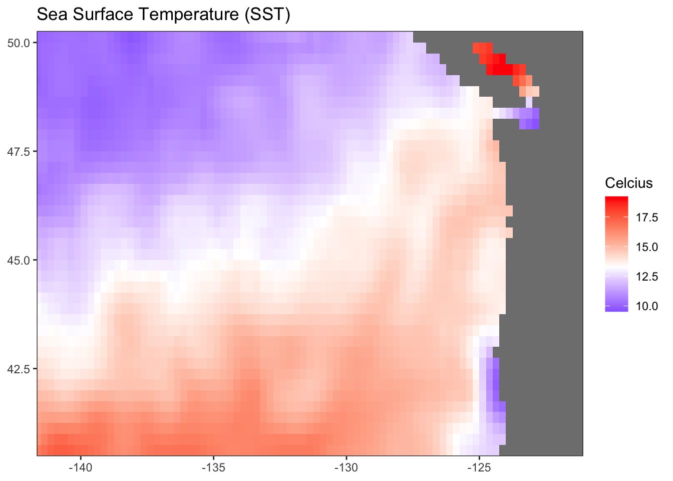

Add a coastline

coast <- rnaturalearth::ne_coastline(scale = 50, returnclass = "sp")
wa_or_coast <- raster::crop(coast, raster::extent(lons[1], lons[2], lats[1], lats[2]))
plot(wa_or_coast)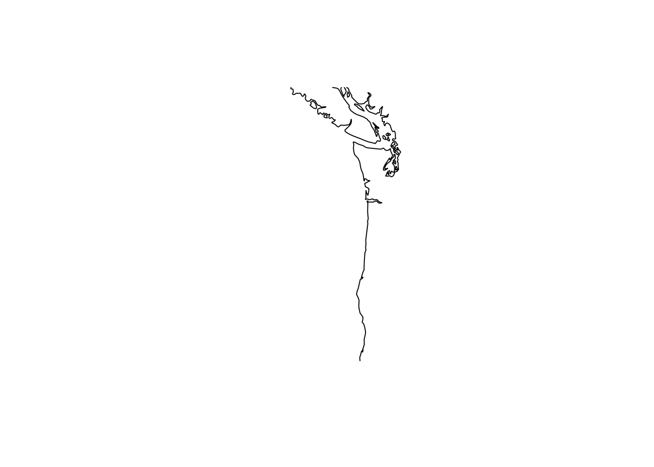

The way that ggplot2 works is to run fortify() on the SpatialLines object to create a data frame. Then we use geom_path() to plot that. But if you look at the coast, you see lots of islands. We need to add grouping to tell geom_path() that there are these groups of paths in the data frame.

gg +
  geom_path(data=wa_or_coast,  aes(x=long,y=lat, grouping=id), size=1, na.rm=TRUE)

Warning: Using `size` aesthetic for lines was deprecated in ggplot2 3.4.0.
ℹ Please use `linewidth` instead.

Warning in geom_path(data = wa_or_coast, aes(x = long, y = lat, grouping =
id), : Ignoring unknown aesthetics: grouping

Warning: Removed 248 rows containing missing values (`geom_raster()`).