Day 18 blue (b)

Code source

Inspired by this https://twitter.com/imagineazhar/status/1593571328484790272 but then I went in a different direction.

Code to download the data

Code

library(marmap)
library(tidyverse)
library(sf)
library(sysfonts)
library(showtext)
library(ggtext)



# ------ Typography ------ 

font_add_google("Mukta", "title_font")
showtext_auto()

title_font <- "title_font"


# ------ Color palette ------ 

palette <- colorRampPalette(c("#03045e", "#0077b6", "#00b4d8",
                              "#90e0ef", "#caf0f8", "#caf0f8"))

# --- Coord

city_coords <- tibble(address = "Seattle, Washington") |> 
  tidygeocoder::geocode(address, method = 'osm', long = long, lat = lat)

long <- city_coords$long[1]
lat <- city_coords$lat[1]

bathmetry <- getNOAA.bathy(lat1 = lat, lat2 = lat+4, lon1 = long, lon2 = long-3, resolution = 1)

df <- fortify.bathy(bathmetry)|>
  filter(z < 0)

Set the bounding box.

Code

crs2 <- 6384 # https://epsg.io/6384

# 10km circle to crop in ----
dist <-  70000
circle <- tibble(long=long-1, lat=lat+1) %>%
  st_as_sf(coords = c("long", "lat"), crs = 4326) %>%
  st_transform(crs = crs2) %>%
  st_buffer(dist = dist) %>%
  st_transform(crs = 4326)

bathy_crop <- df %>%
  st_as_sf(coords = c("x", "y"), crs = 4326) %>%
  st_transform(crs = 4326) %>%
  st_intersection(circle)

Plot code

Code

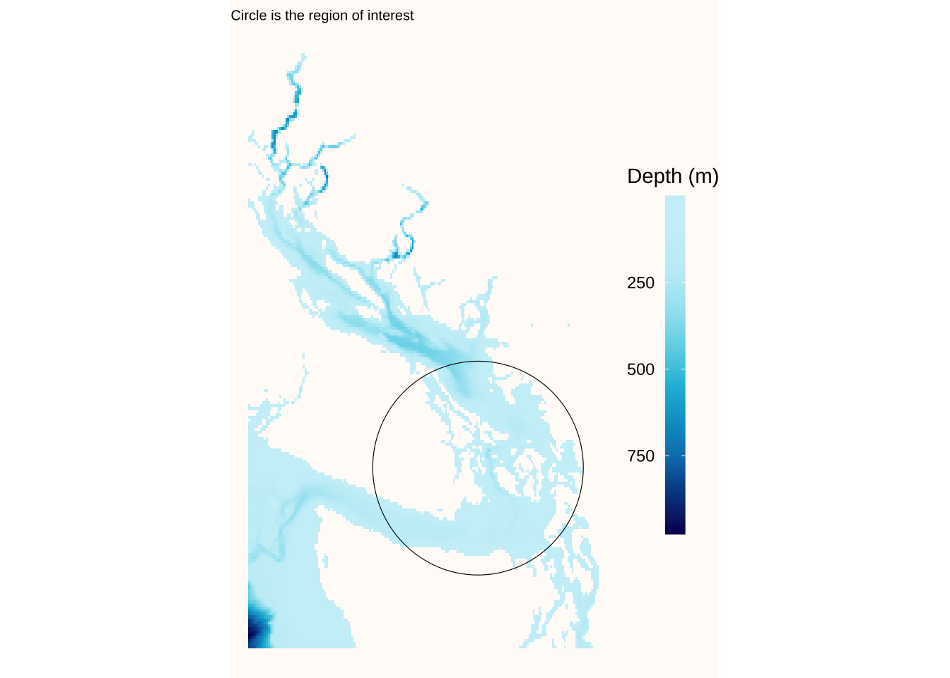
ggplot(df) +
  geom_tile(aes(x = x, y = y, fill = z)) +
  coord_sf(ylim = c(lat, lat+3), xlim = c(long, long-3), expand = FALSE) +
  geom_sf(data = circle, color = "black", fill =  NA) +
  scale_fill_gradientn(colors = palette(10),
                       labels = function(x) format(-x, big.mark = " ", trim = TRUE)) +
  guides(fill = guide_colorbar(label.position = "left", title = "Depth (m)")) +
  theme_void() +
  theme(
    legend.position = "right",
    legend.key.height = unit(2.5, "line"),
    legend.key.width = unit(0.75, "line"),
    plot.background = element_rect(fill = "#FFFBF8", color = NA),
    plot.title = element_markdown(size=7.5)
    ) + 
  ggtitle("Circle is the region of interest")

Coordinate system already present. Adding new coordinate system, which will
replace the existing one.

Code

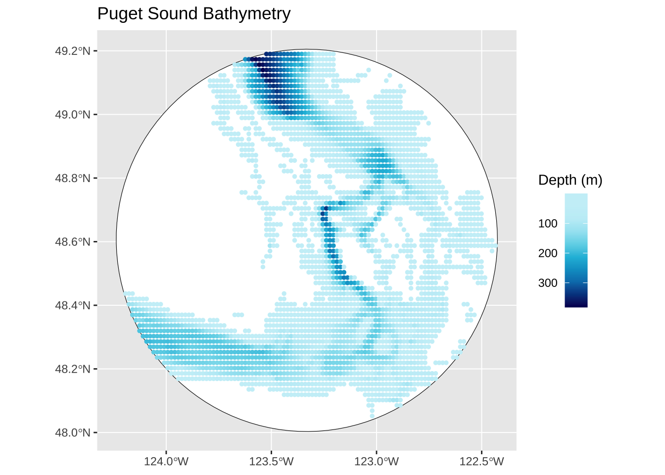
ggplot() +
  geom_sf(data = circle, color = "black", fill =  "white") +
geom_sf(data=bathy_crop, aes(color=z), size=1) +
  ggtitle("Puget Sound Bathymetry") +
scale_color_gradientn(colors = palette(10),
                       labels = function(x) format(-x, big.mark = " ", trim = TRUE)) +
  guides(color = guide_colorbar(label.position = "left", title = "Depth (m)"))