Day 22 Movement

Re-create this image

Today’s goal is to recreate the ARGO float animated image from this blog post: annimate oceanographic data by Masumbuko Semba GitHub

I ended up using more of this code: @HansenDJohnson https://hansenjohnson.org/post/bathymetric-maps-in-r/ and @geokaramanis https://github.com/gkaramanis/30DayMapChallenge/tree/main/2022/07-raster-earth

This will allow me to practice some new skills:

• ARGO float data. I have never worked with that.
• Learn to process netCDF file in R. It’s been awhile since I have done that.
• {gganimate} to animate plots
• Use the {marmap} R package for oceanographic data

Set-up

library(here)
library(tidyverse)
library(stringr)
library(sf)
library(ncdf4)

library(marmap)
library(tidyterra)
library(ggnewscale)
library(gganimate)
library(lubridate)

Download the ARGO data

I went here and downloaded an ARGO float netCDF for a float in the Black Sea. https://dataselection.euro-argo.eu/

ncfile <- here::here("content", "data", "GL_PR_PF_6903766.nc")
argo <- ncdf4::nc_open(ncfile)

Figure out the names of things. Sadly this isn’t a proper ARGO file so oce:read.argo() doesn’t work.

names(argo$var)

 [1] "TIME_QC"                  "POSITION_QC"             
 [3] "DC_REFERENCE"             "DIRECTION"               
 [5] "VERTICAL_SAMPLING_SCHEME" "PRES"                    
 [7] "PRES_QC"                  "TEMP"                    
 [9] "TEMP_QC"                  "PSAL"                    
[11] "PSAL_QC"                 

names(argo$dim)

[1] "TIME"      "DEPTH"     "LATITUDE"  "LONGITUDE" "POSITION"  "STRING32" 
[7] "STRING256"

A bit of poking reveals that the ARGO float data is from 2 sampling schemes: one at the surface and the other that is sampling as the flow goes down. I’ll use just the data from the “Primary sampling” at the surface.

a <- ncdf4::ncvar_get(argo, "VERTICAL_SAMPLING_SCHEME")
good <- stringr::str_detect(a, "Primary sampling")
a[1:3]

[1] "Primary sampling: averaged [10 sec sampling 1 dbar average from surface to 100 dbar; 10 sec sampling 2 dbar average from 100 dbar to 500 dbar; 10 sec sampling 5 dbar average from 500 dbar to 1000 dbar]" 
[2] "Primary sampling: averaged [10 sec sampling 5 dbar average from 2000 dbar to 500 dbar; 10 sec sampling 2 dbar average from 500 dbar to 100 dbar; 10 sec sampling 1 dbar average from 100 dbar to 2.4 dbar]"
[3] "Near-surface sampling: averaged unpumped [10 sec sampling 1 dbar average from 2.4 dbar to surface]"                                                                                                        

Next I notice that the time is in julian days so I will need to convert that. There are a few ways to convert julian to date/time. Making the origin date a POSIXlt date object and adding on the seconds is an easy way.

# print(argo) and you'll see the ref time
to <- as.POSIXlt("1950-01-01")

argo_df <- tibble(
  time = ncvar_get(argo, "TIME"),
  lon = ncvar_get(argo, "LONGITUDE"),
  lat = ncvar_get(argo, "LATITUDE"),
  temp = ncvar_get(argo, "TEMP")[1,],
  psal = ncvar_get(argo, "PSAL")[1,]
) %>% subset(good) %>%
  mutate(date = to+time*60*60*24) %>% # need to convert time to secs
  mutate(qtr = as.character(quarter(date)))

Black Sea

Using https://www.latlong.net/, I grabbed box coordinates.

y <- c(39, 47)
x <- c(26, 44)

Make the bathymetry plot

Get bathymetry.

bathy <- marmap::getNOAA.bathy(x[1], x[2], y[1], y[2], resolution = 3)

Querying NOAA database ...

This may take seconds to minutes, depending on grid size

Building bathy matrix ...

bathy_df <- marmap::fortify.bathy(bathy)

autoplot.bathy(bathy, geom=c("tile","contour")) +
    scale_fill_gradient2(low="dodgerblue4", mid="gainsboro", high="darkgreen")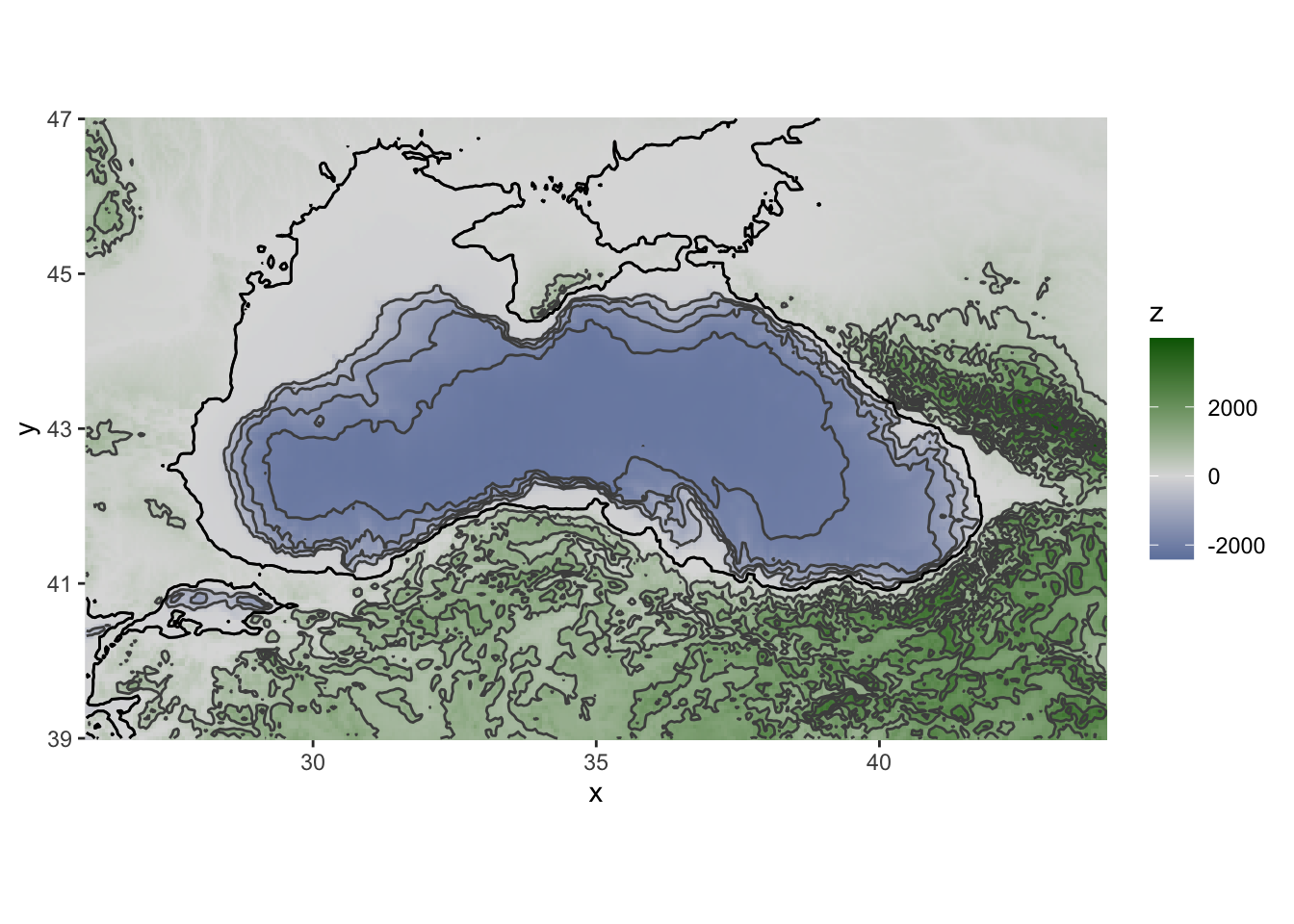

Map a map with the ARGO data added.

basemap <- ggplot() +
  # water raster
  geom_raster(data = bathy_df %>% filter(z < 0), aes(x, y, fill = z), show.legend=FALSE) +
  scale_fill_hypso_c("etopo1_bathy") +
  # add contours
  geom_contour(data = bathy_df %>% filter(z < 0), 
               aes(x=x, y=y, z=z),
               breaks=c(-100),
               linewidth=c(0.3),
               colour="grey") +
  geom_contour(data = bathy_df %>% filter(z < 0), 
               aes(x=x, y=y, z=z),
               breaks=c(-500, -1000, -1500, -2000),
               linewidth=c(0.3),
               colour="white") +
  new_scale_fill() +
  # Add argo points
  geom_point(data = argo_df, aes(x = lon, y = lat, color = temp), size=3) +
  scale_colour_steps2(low = "blue", mid = "white", high = "red",
    midpoint = mean(argo_df$temp), name="temperature (C)") +
  new_scale_fill() +
  # land raster
  geom_raster(data = bathy_df %>% filter(z >= 0), aes(x, y, fill = z), show.legend=FALSE) +
  scale_fill_hypso_c("gmt_globe_hypso") +
  theme_void() +
  theme(
    legend.position = "bottom"
  ) + 
  ggtitle("An Argo bouy in the Black Sea")
basemap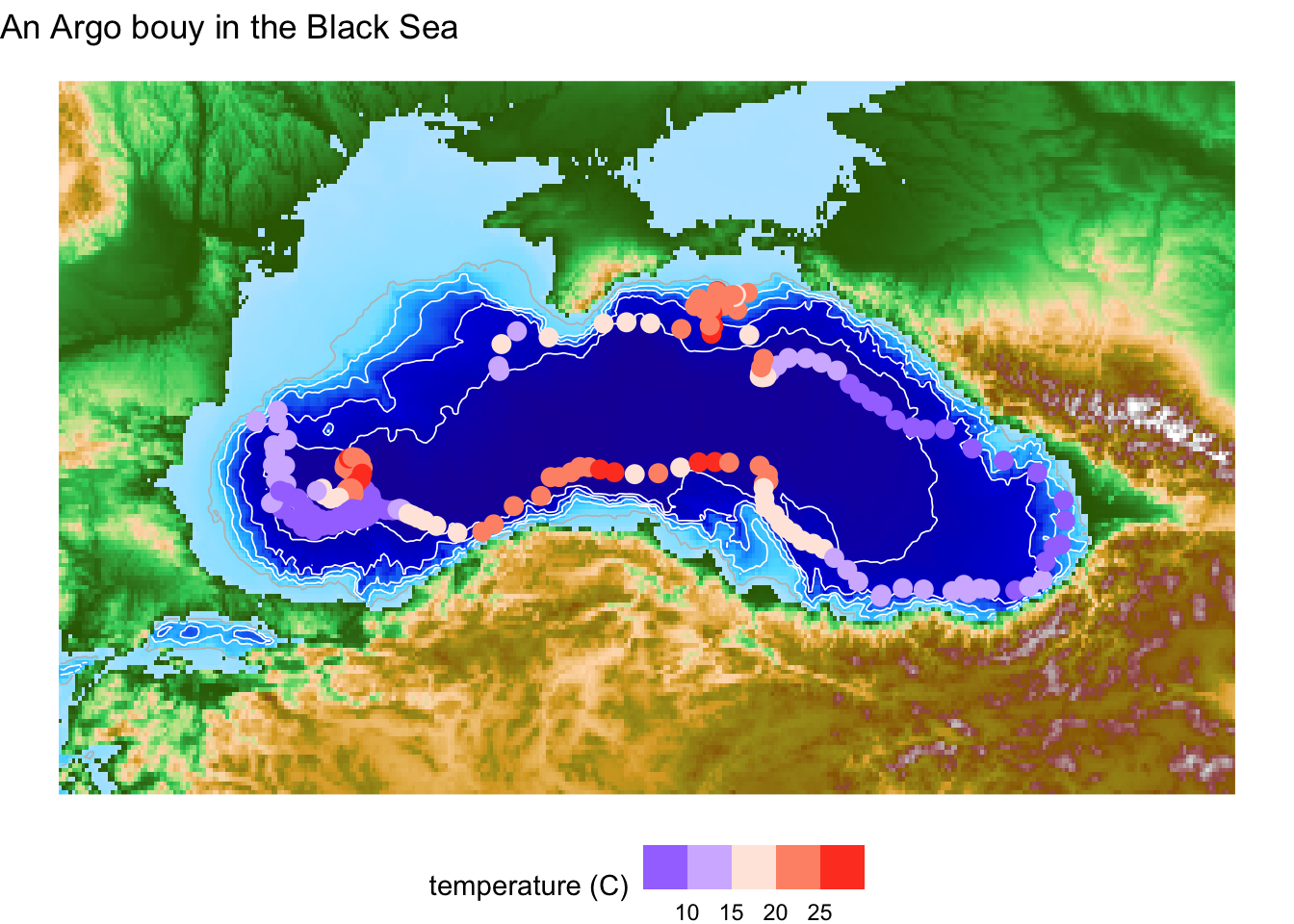

## map the location
argo.animate <- basemap +
 geom_label(
    data = argo_df %>% slice(seq(1,dim(argo_df)[1],14)),
    aes(label = format(date, "%b %Y")), x=35, y=43)+
  transition_time(date)+
  ease_aes("sine-in-out")+
  shadow_mark()

gganimate::animate(argo.animate)

Save

gganimate::anim_save(here::here("content", "argo.gif"))