Day 19 globe

Code source inspriation

• https://twitter.com/ryanahart/status/1593966022553489410
• https://twitter.com/dhernangomez/status/1591710364571504640
• https://twitter.com/geokaramanis/status/1593999504323317760
• https://github.com/curatedmess/30DayMapChallenge/blob/main/2022/11192022/qatar.R

But see this globe by @geokaramanis for the Day 7 raster entry https://github.com/gkaramanis/30DayMapChallenge/tree/main/2022/07-raster-earth

Code to download the data

The basic libraries

library(tidyverse)
library(sf)

Get the Seattle lat/lon

Code

# Center
city_coords <- tibble(address = "Seattle, Washington") |> 
  tidygeocoder::geocode(address, method = 'osm', long = long, lat = lat)
long <- city_coords$long[1]
lat <- city_coords$lat[1]
crs2 <- 6384 # https://epsg.io/6384
coord_center <-
  tibble(long, lat) %>%
  sf::st_as_sf(coords = c("long", "lat"), crs = 4326)

Set the projection. Had to futz a bit to get something that was close and didn’t throw an error w ggplot.

crs_string <- paste0("+proj=ortho +lat_0=", lat, " +lon_0=", long)
# crs_string <- "+proj=ortho +lat_0=45 +lon_0=-105"

Get US elevations and define hill shading. This will be spatraster and comes with a projection which you can check with terra::crs(). We don’t need to change that; just need to know that it is specified.

Code

library(tidyterra) # for geom_spatraster
library(geodata)
library(scales)
r <- geodata::elevation_global(res=10, path = tempdir())
names(r) <- "alt"

slope <- terra::terrain(r, "slope", unit = "radians")
aspect <- terra::terrain(r, "aspect", unit = "radians")
hill <- terra::shade(slope, aspect, 30, 270)

# give the hill shading a name so I can refer to it in aes()
names(hill) <- "shades"

Create a blue globe that will represent the ocean. 637100 is the radius of the earth in meters.

Code

# these are sf functions
ocean <- st_point(x = c(0,0)) %>%
  st_buffer(dist = 6371000) %>%
  st_sfc(crs = crs_string)

Plot code

Create my globe. The palette “dem_poster” comes from tidyterra package.

Code

library(ggfx) # for with_shadow
p1 <- ggplot() +
  with_shadow(geom_sf(data = ocean, fill = "#BBDEFB", color = NA), sigma = 30, x_offset = 25, y_offset = 25, color = "#58595d") +
  geom_spatraster(data = hill, aes(fill=shades), maxcell = Inf) +
  geom_spatraster(data=r, maxcell = Inf) +
  scale_fill_hypso_tint_c(limits = as.vector(minmax(r)), 
                          palette = "dem_poster",
                          alpha =0.8,
                          labels = scales::label_comma(),
                          breaks = c(seq(0,1000, 250), seq(2000, 6000, 1000))) +
  guides(fill=guide_legend(title = "elevation", reverse = TRUE)) +
  coord_sf(crs = crs_string) +
  theme_void()
p1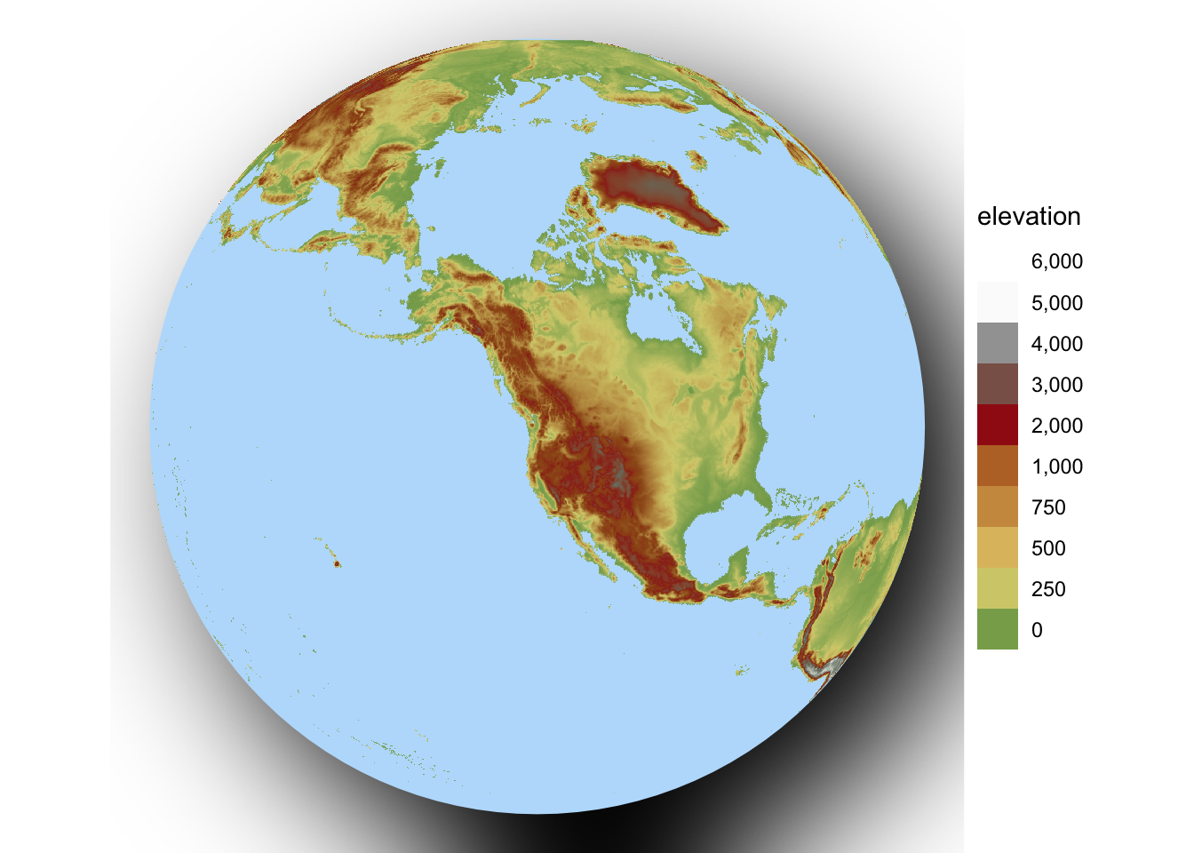

Then add some annotation. The x and y units are in meters, so the nudge has to be huge (millions).

Code

library("ggrepel")
p2 <- p1 + geom_sf(data=coord_center) + 
  geom_text_repel(data = coord_center, aes(x=st_coordinates(coord_center)[1], y=st_coordinates(coord_center)[2]), label="Seattle", 
        nudge_x = -3371000, nudge_y = -1371000) +
  labs(
    title = "Globe with elevations",
    caption = "Graphic: EE Holmes"
  ) +
  theme(
    plot.background = element_rect(fill = "grey97", color = NA),
    plot.margin = unit(c(.5,.5,.5,.5), "cm"),
    plot.title = element_text(hjust = 0.045, size = 26, face = "bold")
  )
p2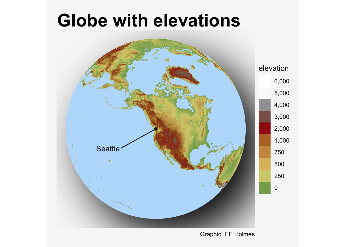

Swap out that square background with one with rounded corners. Well this didn’t really work since I couldn’t figure out how to save.

Code

library(grid)
g <- ggplotGrob(p2)
bg <- g$grobs[[1]]
round_bg <- roundrectGrob(x=bg$x, y=bg$y, width=bg$width, height=bg$height,
                          r=unit(0.1, "snpc"),
                          just=bg$just, name=bg$name, gp=bg$gp, vp=bg$vp)
g$grobs[[1]] <- round_bg
grid.draw(g)

For some reason the shadowing looks wrong in the html. Looks like this in the saved image:

knitr::include_graphics(here::here("content", "globe_elevation.png"))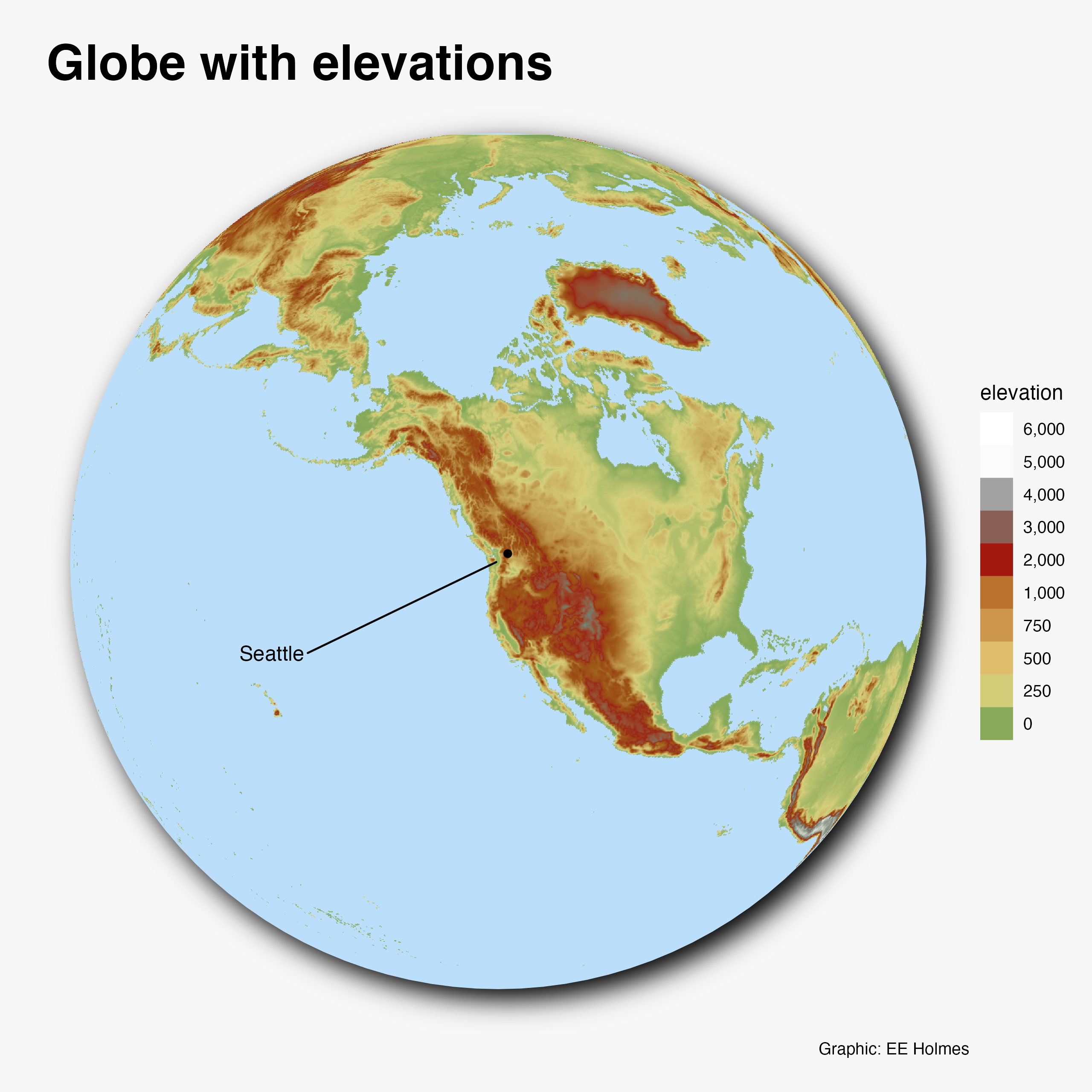

Save image

ggsave(paste0("globe_elevation", ".png"), dpi = 320, width = 8, height = 8)