Day 20 favorite

Code source inspriation

A course I took on Species Distribution modeling (sdm). I wrote up my course project into a bookdown book. This was my first foray into making maps in R. https://eeholmes.github.io/Species-Dist-Modeling—Trillium/

Link to just the R code for map

Set-up Vermont and New Hampshire boundaries

There is surely an easier way to do this.

library(sp)
library(raster)
library(maps)

First I need to define an raster::extent object for a box bounding NH and VT.

NHVT <- raster::extent(-73.61056, -70.60205, 42.48873, 45.37969)

I download the shapefile for the NH and VT state borders using getData() which gives polygons for countries. Level 1 will be the state boundaries (I assume). The shape file has all the states. Then I use subset() to get the two states that I want. path says where to save the downloaded file.

usashp <- raster::getData('GADM', country='USA', level=1, path="data")
nhvtshp <- subset(usashp, NAME_1 %in% c("New Hampshire", "Vermont"))

Check the projection for this shapefile:

crs(nhvtshp)

I can plot the shapes.

plot(nhvtshp, border="blue", axes=TRUE)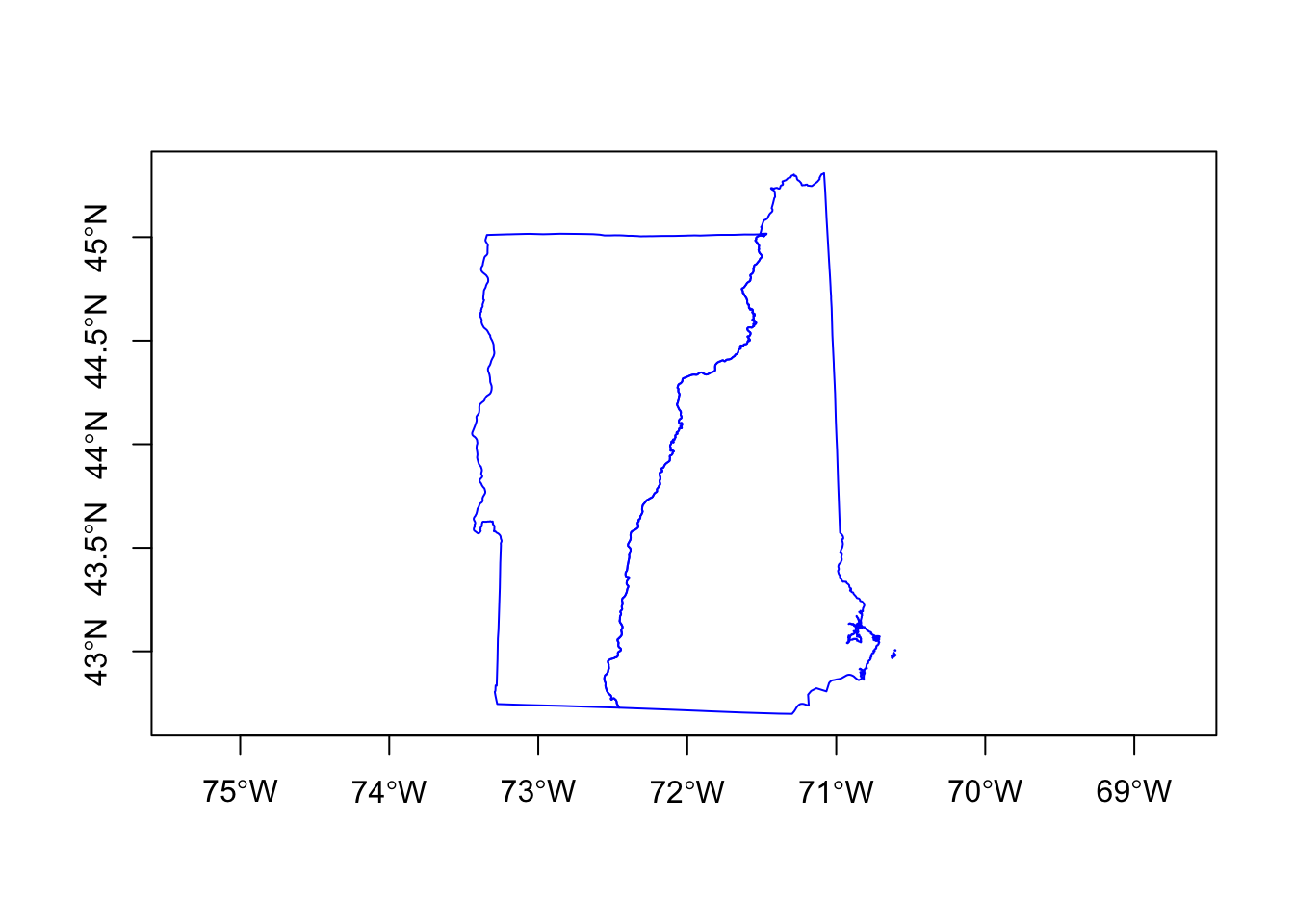

I save the shapefile data to a file so I can use it later.

save(nhvtshp, NHVT, file=here::here("content", "data", 
"shapefiles.RData"))

Download Trillium records

This map will use the following libraries:

library(dismo) # as sdm package
library(sp)
library(here)

Load the shapefiles created earlier.

load(file=here::here("content", "data", 
"shapefiles.RData"))

Download records

I will download occurrence data for Trillium grandiflorum and Trillium undulatum in my NHVT bounding box from the Global Biodiversity Information Facility. nrecs seems to be ignored. geo means only points with longitude and latitude. removeZeros means get rid of NA in location. ext is the bounding box to use.

First I set where I will save the file and check if it is already there. I do this because if I rerun this script, I don’t want to re-download. Note that GBIF data is updated weekly so using a time-stamp on your file might be good, but I am not doing that for this example.

filePath <- here::here("content", "data", "trillium_presences.RData")

Now I download if I haven’t downloaded already because this takes awhile. The downloaded data has many columns that I don’t need. I will subset the following columns. select in the subset() call says what columns to use.

if (!file.exists(filePath)) {
  # Download
  grandiflorum <- dismo::gbif("Trillium",
    species = "grandiflorum",
    nrecs = 300, geo = TRUE,
    removeZeros = TRUE, ext = NHVT
  )
  undulatum <- dismo::gbif("Trillium",
    species = "undulatum",
    nrecs = 300, geo = TRUE,
    removeZeros = TRUE, ext = NHVT
  )
  # select columns
  colsWeNeed <- c("species", "lat", "lon", "locality", "year", "coordinateUncertaintyInMeters", "occurrenceID", "occurrenceRemarks", "geodeticDatum")
  grandiflorum <- subset(grandiflorum, select = colsWeNeed)
  undulatum <- subset(undulatum, select = colsWeNeed)
  trillium.raw <- rbind(grandiflorum, undulatum)
  save(trillium.raw, file = filePath)
}

Load in the presences data (saved from code above).

load(filePath)

Check the projection to make sure it makes sense and there is only one value. Check that it is the same projection as my other layers.

unique(trillium.raw$geodeticDatum) # "WGS84"

[1] "WGS84"

trillium.raw is just a data frame. I make it a sp object (specifically a SpatialPointsDataFrame) using sp::coordinates() to specify which columns are the longitude and latitude.

trillium <- trillium.raw
sp::coordinates(trillium) <- c("lon", "lat")

Check that it looks ok and there are no NAs.

summary(trillium$lon)

   Min. 1st Qu.  Median    Mean 3rd Qu.    Max. 
 -73.61  -73.01  -72.57  -72.38  -71.73  -70.60 

summary(trillium$lat)

   Min. 1st Qu.  Median    Mean 3rd Qu.    Max. 
  42.49   43.61   44.18   44.00   44.47   45.38 

The coordinateUncertaintyInMeters column give the uncertainty of the observation location. Some of the uncertainties are huge and I don’t want those.

table(cut(trillium$coordinateUncertaintyInMeters, c(0, 200, 500, 1000, 2000, 5000)))

      (0,200]     (200,500]   (500,1e+03] (1e+03,2e+03] (2e+03,5e+03] 
         3131           142            92            87           118 

I am going to keep only those locations with a location accuracy within 200m.

good <- which(trillium$coordinateUncertaintyInMeters < 200)
trillium <- trillium[good, ]

Plot the locations

Now I can plot the occurrences points and add the NH and VT state boundaries. Trillium undulatum is much more common.

plot(nhvtshp, border = "blue", axes = TRUE)
plot(subset(trillium, species == "Trillium grandiflorum"), pch = 19, cex = 0.25, add = TRUE)
plot(subset(trillium, species == "Trillium undulatum"), pch = 19, cex = 0.25, col = "red", add = TRUE)
title("Trillium grandiflorum (black) and Trillium undulatum (red) records", cex.main=0.75)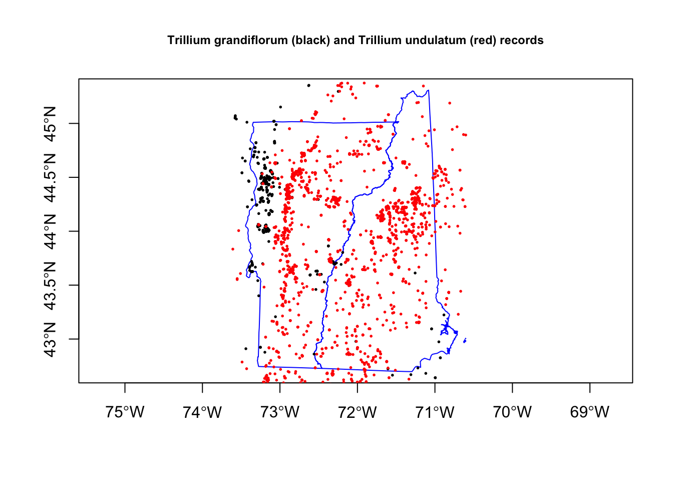

Save

png(file = "day20_trillium.png", bg = "white")
plot(nhvtshp, border = "blue", axes = TRUE)
plot(subset(trillium, species == "Trillium grandiflorum"), pch = 19, cex = 0.25, add = TRUE)
plot(subset(trillium, species == "Trillium undulatum"), pch = 19, cex = 0.25, col = "red", add = TRUE)
title("Trillium grandiflorum (black) and Trillium undulatum (red) records", cex.main=1)
dev.off()