Day 2 Lines

Re-create this image

https://milospopovic.net/mapping-wind-data-in-r/ using his code. I made some changes to the code but it is largely adapted and copied from Milos Popovic 2022/08/28.

This uses the {metR} package function geom_streamline() to plot the lines. Nice blog on using this for wind and current plot here: Plotting streamlines by Masumbuko Semba.

Set up

Install packages.

# libraries we need
libs <- c(
  "tidyverse", "sf", "giscoR",
  "lubridate", "classInt",
  "rWind", "metR", "oce", "tidyterra"
)

# install missing libraries
installed_libs <- libs %in% rownames(installed.packages())
if (any(installed_libs == F)) {
  install.packages(libs[!installed_libs])
}

# load libraries
invisible(lapply(libs, library, character.only = T))

Specifications for date and location.

year <- 2022
month <- c(start = 8, end = 8)
day <- c(start = 27, end = 28)
by <- "1 hours"
latlon <- c(xmin = -28.5, xmax = 58.5, ymin = 34.0, ymax = 73.5)

Get wind function

get_wind_data <- function(time_range, mean_wind_data, eur_wind_df) {
  time_range <- seq(lubridate::ymd_hms(paste(year, month[1], day[1], 00, 00, 00, sep = "-")),
    lubridate::ymd_hms(paste(year, month[2], day[2], 00, 00, 00, sep = "-")),
    by = by
  )

  mean_wind_data <- rWind::wind.dl_2(time_range, latlon[1], latlon[2], latlon[3], latlon[4]) %>%
    rWind::wind.mean()

  df <- as.data.frame(mean_wind_data)
  return(df)
}

Get wind data and make into a raster for plotting later.

crs_string <- "+proj=longlat +datum=WGS84 +no_defs"
filePath <- here::here("content", "data", paste0("wind-", year, "-", month[1], "-", day[1], ".RData"))
if (!file.exists(filePath)) {
  df <- get_wind_data()
  save(df, file = filePath)
} else {
  load(filePath)
}
colnames(df) <- c("time", "lat", "lon", "u", "v", "dir", "vel")
df2 <- data.frame(x = df$lon, y = df$lat, z = df$vel)
ras <- raster::rasterFromXYZ(df2, crs = crs_string)
bb <- st_bbox(ras)
library(terra)
r <- terra::rast(ras)
names(r) <- "vel"
setMinMax(r)

Get the land polygons.

region <- c("Europe", "Asia")
land_sf <- giscoR::gisco_get_countries(
  year = "2016", epsg = "4326",
  resolution = "10", region = region
)

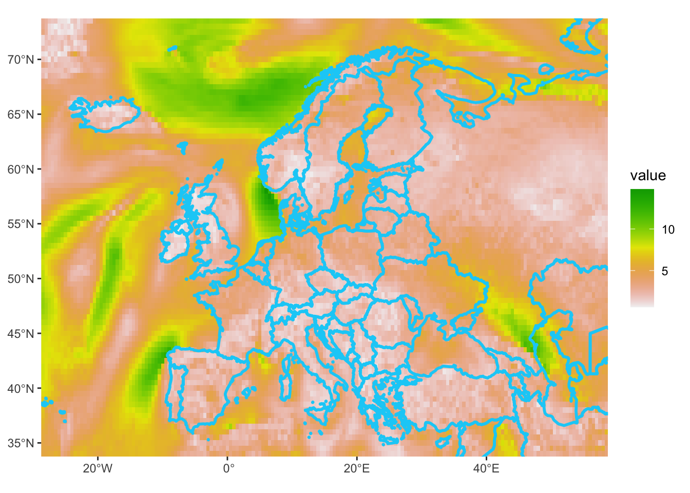
Test plot of the raster of wind speed.

autoplot(r) +
  geom_sf(
    data = land_sf,
    fill = NA,
    color = "#07CFF7",
    linewidth = 1,
    alpha = .99
  ) +
  coord_sf(
    crs = crs_string,
    xlim = c(bb["xmin"], bb["xmax"]),
    ylim = c(bb["ymin"], bb["ymax"]),
    expand = FALSE
  )

Set up colors for lines and the legend.

# colors
cols <- c(
  "#feebe2", "#d84594", "#bc2b8a", "#7a0177"
)

newcol <- colorRampPalette(cols)
ncols <- 6
cols2 <- newcol(ncols)

# breaks
vmin <- min(df$vel, na.rm = T)
vmax <- max(df$vel, na.rm = T)

brk <- classInt::classIntervals(df$vel,
  n = 6,
  style = "fisher"
)$brks %>%
  head(-1) %>%
  tail(-1) %>%
  append(vmax)

Warning in classInt::classIntervals(df$vel, n = 6, style = "fisher"): N is
large, and some styles will run very slowly; sampling imposed

breaks <- c(vmin, brk)

Make the plot. the after_stat() bit is to delay the calculation of the color until after geom_streamline() does some grouping, I think. Anyhow just using color = sqrt(vel) doesn’t work. I am not sure where the size warning is coming from since I don’t use it in any aes(). Maybe from geom_streamline()?

p <- df %>%
  ggplot() +
  geom_sf(
    data = land_sf,
    fill = "grey90",
    color = "#07CFF7",
    linewidth = .5,
    alpha = .99
  ) +
  metR::geom_streamline(
    data = df,
    aes(
      x = lon, y = lat, dx = u, dy = v,
      color = sqrt(after_stat(dx)^2 + after_stat(dy)^2)
    ),
    L = 2, res = 2, n = 60,
    arrow = NULL, lineend = "round",
    alpha = .85
  ) +
  geom_sf(
    data = land_sf,
    fill = NA,
    color = "#07CFF7",
    linewidth = .5,
    alpha = .5
  ) +
  coord_sf(
    crs = crs_string,
    xlim = c(bb["xmin"], bb["xmax"]),
    ylim = c(bb["ymin"], bb["ymax"]),
    expand = FALSE
  ) +
  scale_color_gradientn(
    name = "Average speed (m/s)",
    colours = cols2,
    breaks = breaks,
    labels = round(breaks, 1),
    limits = c(vmin, vmax)
  ) +
  guides(
    fill = "none",
    color = guide_legend(
      direction = "horizontal",
      keyheight = unit(2.5, units = "mm"),
      keywidth = unit(15, units = "mm"),
      title.position = "top",
      title.hjust = .5,
      label.hjust = .5,
      nrow = 1,
      byrow = T,
      reverse = F,
      label.position = "bottom"
    )
  ) +
  theme_bw() +
  theme(legend.position = c(.5, .1))
p

Warning: Using the `size` aesthetic in this geom was deprecated in ggplot2 3.4.0.
ℹ Please use `linewidth` in the `default_aes` field and elsewhere instead.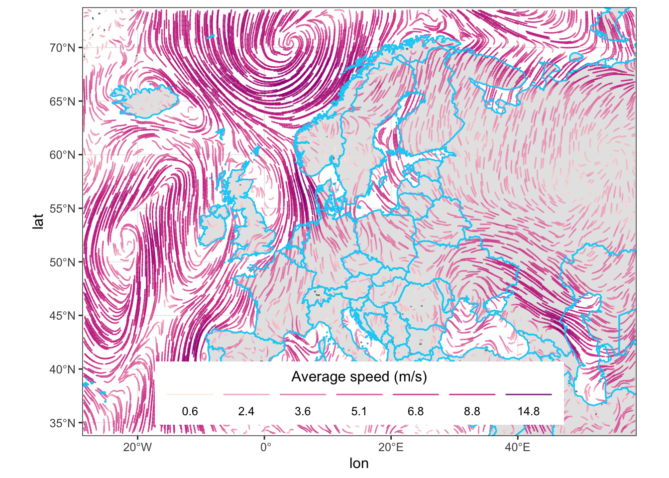

axissize <- 30
p2 <- p +
  theme(
    axis.text.x = element_text(size = axissize),
    axis.text.y = element_text(size = axissize),
    axis.title.x = element_text(size = axissize),
    axis.title.y = element_text(size = axissize),
    legend.text = element_text(size = 60, color = "black"),
    legend.title = element_text(size = 80, color = "black"),
    legend.key = element_blank(),
    legend.spacing.y = unit(.5, "pt"),
  )
ggsave(
  filename = "eur_wind.png",
  width = 8.5, height = 7, dpi = 300, p2
)